Tutorial for mapping data with Tangram

by Tommaso Biancalani biancalt@gene.com and Ziqing Lu luz21@gene.com

• The notebook introduces to mapping single cell data on spatial data using the Tangram method.

• The notebook uses data from mouse brain cortex (different than those adopted in the manuscript).

Last changelog

• June 13th - Tommaso Biancalani biancalt@gene.com

---

Installation

• Make sure tangram-sc is installed via pip install tangram-sc.

• Otherwise, edit and uncomment the line starting with sys.path specifying the Tangram folder.

• The Python environment needs to install the packages listed in environment.yml.

import os, sys
import numpy as np
import pandas as pd
import matplotlib.pyplot as plt
import seaborn as sns
import scanpy as sc
import torch
sys.path.append('./')  # uncomment for local import
import tangram as tg

%load_ext autoreload
%autoreload 2
%matplotlib inline

tg.__version__

'1.0.0'

---

Download the data

• If you have wget installed, you can run the following code to automatically download and unzip the data.

# Skip this cells if data are already downloaded
!wget https://storage.googleapis.com/tommaso-brain-data/tangram_demo/mop_sn_tutorial.h5ad.gz -O data/mop_sn_tutorial.h5ad.gz
!wget https://storage.googleapis.com/tommaso-brain-data/tangram_demo/slideseq_MOp_1217.h5ad.gz -O data/slideseq_MOp_1217.h5ad.gz
!wget https://storage.googleapis.com/tommaso-brain-data/tangram_demo/MOp_markers.csv -O data/MOp_markers.csv
!gunzip -f data/mop_sn_tutorial.h5ad.gz
!gunzip -f data/slideseq_MOp_1217.h5ad.gz

--2021-11-03 14:35:06--  https://storage.googleapis.com/tommaso-brain-data/tangram_demo/mop_sn_tutorial.h5ad.gz
Resolving storage.googleapis.com (storage.googleapis.com)... 172.217.6.48, 172.217.6.80, 142.250.72.208, ...
Connecting to storage.googleapis.com (storage.googleapis.com)|172.217.6.48|:443... connected.
HTTP request sent, awaiting response... 200 OK
Length: 474724402 (453M) [application/x-gzip]
Saving to: ‘data/mop_sn_tutorial.h5ad.gz’

100%[======================================>] 474,724,402  123MB/s   in 3.8s

2021-11-03 14:35:10 (118 MB/s) - ‘data/mop_sn_tutorial.h5ad.gz’ saved [474724402/474724402]

--2021-11-03 14:35:10--  https://storage.googleapis.com/tommaso-brain-data/tangram_demo/slideseq_MOp_1217.h5ad.gz
Resolving storage.googleapis.com (storage.googleapis.com)... 172.217.6.48, 172.217.6.80, 142.250.72.208, ...
Connecting to storage.googleapis.com (storage.googleapis.com)|172.217.6.48|:443... connected.
HTTP request sent, awaiting response... 200 OK
Length: 12614106 (12M) [application/x-gzip]
Saving to: ‘data/slideseq_MOp_1217.h5ad.gz’

100%[======================================>] 12,614,106  --.-K/s   in 0.1s

2021-11-03 14:35:11 (116 MB/s) - ‘data/slideseq_MOp_1217.h5ad.gz’ saved [12614106/12614106]

--2021-11-03 14:35:11--  https://storage.googleapis.com/tommaso-brain-data/tangram_demo/MOp_markers.csv
Resolving storage.googleapis.com (storage.googleapis.com)... 172.217.6.48, 172.217.6.80, 142.250.72.208, ...
Connecting to storage.googleapis.com (storage.googleapis.com)|172.217.6.48|:443... connected.
HTTP request sent, awaiting response... 200 OK
Length: 2510 (2.5K) [text/csv]
Saving to: ‘data/MOp_markers.csv’

100%[======================================>] 2,510       --.-K/s   in 0s

2021-11-03 14:35:11 (13.0 MB/s) - ‘data/MOp_markers.csv’ saved [2510/2510]

• If you do not have wget installed, manually download data from the links below:

  • snRNA-seq datasets collected from adult mouse cortex: 10Xv3 MOp.

  • For spatial data, we will use one coronal slice of Slide-seq2 data (adult mouse brain; MOp area).

  • We will map them via a few hundred marker genes, found in literature.

  • All datasets need to be unzipped: resulting h5ad and csv files should be placed in the data folder.

---

Load spatial data

• Spatial data need to be organized as a voxel-by-gene matrix. Here, Slide-seq data contains 9852 spatial voxels, in each of which there are 24518 genes measured.

path = os.path.join('./data', 'slideseq_MOp_1217.h5ad')
ad_sp = sc.read_h5ad(path)
ad_sp

AnnData object with n_obs × n_vars = 9852 × 24518
    obs: 'orig.ident', 'nCount_RNA', 'nFeature_RNA', 'x', 'y'

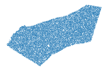
• The voxel coordinates are saved in the fields obs.x and obs.y which we can use to visualize the spatial ROI. Each “dot” is the center of a 10um voxel.

xs = ad_sp.obs.x.values
ys = ad_sp.obs.y.values
plt.axis('off')
plt.scatter(xs, ys, s=.7);
plt.gca().invert_yaxis()

---

Single cell data

• By single cell data, we generally mean either scRNAseq or snRNAseq.

• We start by mapping the MOp 10Xv3 dataset, which contains single nuclei collected from a posterior region of the primary motor cortex.

• They are approximately 26k profiled cells with 28k genes.

path = os.path.join('data','mop_sn_tutorial.h5ad')
ad_sc = sc.read_h5ad(path)
ad_sc

AnnData object with n_obs × n_vars = 26431 × 27742
    obs: 'QC', 'batch', 'class_color', 'class_id', 'class_label', 'cluster_color', 'cluster_labels', 'dataset', 'date', 'ident', 'individual', 'nCount_RNA', 'nFeature_RNA', 'nGene', 'nUMI', 'project', 'region', 'species', 'subclass_id', 'subclass_label'
    layers: 'logcounts'

• Usually, we work with data in raw count form, especially if the spatial data are in raw count form as well.

• If the data are in integer format, that probably means they are in raw count.

np.unique(ad_sc.X.toarray()[0, :])

array([  0.,   1.,   2.,   3.,   4.,   5.,   6.,   7.,   8.,   9.,  10.,
        11.,  12.,  13.,  14.,  15.,  16.,  17.,  18.,  19.,  20.,  21.,
        22.,  23.,  24.,  25.,  26.,  27.,  28.,  29.,  30.,  31.,  33.,
        34.,  36.,  39.,  40.,  43.,  44.,  46.,  47.,  49.,  50.,  53.,
        56.,  57.,  58.,  62.,  68.,  69.,  73.,  77.,  80.,  85.,  86.,
        98., 104., 105., 118., 121., 126., 613.], dtype=float32)

• Here, we only do some light pre-processing as library size correction (in scanpy, via sc.pp.normalize) to normalize the number of count within each cell to a fixed number.

• Sometimes, we apply more sophisticated pre-processing methods, for example for batch correction, although mapping works great with raw data.

• Ideally, the single cell and spatial datasets, should exhibit signals as similar as possible and the pre-processing pipeline should be finalized to harmonize the signals.

sc.pp.normalize_total(ad_sc)

• It is a good idea to have annotations in the single cell data, as they will be projected on space after we map.

• In this case, cell types are annotated in the subclass_label field, for which we plot cell counts.

• Note that cell type proportion should be similar in the two datasets: for example, if Meis is a rare cell type in the snRNA-seq then it is expected to be a rare one even in the spatial data as well.

ad_sc.obs.subclass_label.value_counts()

L5 IT        5623
Oligo        4330
L2/3 IT      3555
L6 CT        3118
Astro        2600
Micro-PVM    1121
Pvalb         972
L6 IT         919
L5 ET         903
L5/6 NP       649
Sst           627
Vip           435
L6b           361
Endo          357
Lamp5         332
VLMC          248
Peri          187
Sncg           94
Name: subclass_label, dtype: int64

---

Prepare to map

• Tangram learns a spatial alignment of the single cell data so that the gene expression of the aligned single cell data is as similar as possible to that of the spatial data.

• In doing this, Tangram only looks at a subset genes, specified by the user, called the training genes.

• The choice of the training genes is a delicate step for mapping: they need to bear interesting signals and to be measured with high quality.

• Typically, a good start is to choose 100-1000 top marker genes, evenly stratified across cell types. Sometimes, we also use the entire transcriptome, or perform different mappings using different set of training genes to see how much the result change.

• For this case, we choose 253 marker genes of the MOp area which were curated in a different study.

df_genes = pd.read_csv('data/MOp_markers.csv', index_col=0)
markers = np.reshape(df_genes.values, (-1, ))
markers = list(markers)
len(markers)

253

• We now need to prepare the datasets for mapping by creating training_genes field in uns dictionary of the two AnnData structures.

• This training_genes field contains genes subset on the list of training genes. This field will be used later inside the mapping function to create training datasets.

• Also, the gene order needs to be the same in the datasets. This is because Tangram maps using only gene expression, so the \(j\)-th column in each matrix must correspond to the same gene.

• And if data entries of a gene are all zero, this gene will be removed

• This task is performed by the helper pp_adatas.

tg.pp_adatas(ad_sc, ad_sp, genes=markers)

INFO:root:249 training genes are saved in `uns``training_genes` of both single cell and spatial Anndatas.
INFO:root:18000 overlapped genes are saved in `uns``overlap_genes` of both single cell and spatial Anndatas.
INFO:root:uniform based density prior is calculated and saved in `obs``uniform_density` of the spatial Anndata.
INFO:root:rna count based density prior is calculated and saved in `obs``rna_count_based_density` of the spatial Anndata.

• You’ll now notice that the two datasets now contain 249 genes, but 253 markers were provided.

• This is because the marker genes need to be shared by both dataset. If a gene is missing, pp_adatas will just take it out.

• Finally, the assert line below is a good way to ensure that the genes in the training_genes field in uns are actually ordered in both AnnDatas.

ad_sc

AnnData object with n_obs × n_vars = 26431 × 26496
    obs: 'QC', 'batch', 'class_color', 'class_id', 'class_label', 'cluster_color', 'cluster_labels', 'dataset', 'date', 'ident', 'individual', 'nCount_RNA', 'nFeature_RNA', 'nGene', 'nUMI', 'project', 'region', 'species', 'subclass_id', 'subclass_label'
    var: 'n_cells'
    uns: 'training_genes', 'overlap_genes'
    layers: 'logcounts'

ad_sp

AnnData object with n_obs × n_vars = 9852 × 20864
    obs: 'orig.ident', 'nCount_RNA', 'nFeature_RNA', 'x', 'y', 'uniform_density', 'rna_count_based_density'
    var: 'n_cells'
    uns: 'training_genes', 'overlap_genes'

assert ad_sc.uns['training_genes'] == ad_sp.uns['training_genes']

---

Map

• We can now train the model (ie map the single cell data onto space).

• Mapping should be interrupted after the score plateaus,which can be controlled by passing the num_epochs parameter.

• The score measures the similarity between the gene expression of the mapped cells vs spatial data: higher score means better mapping.

• Note that we obtained excellent mapping even if Tangram converges to a low scores (the typical case is when the spatial data are very sparse): we use the score merely to assess convergence.

• If you are running Tangram with a GPU, uncomment device=cuda:0 and comment the line device=cpu. On a MacBook Pro 2018, it takes ~1h to run. On a P100 GPU it should be done in a few minutes.

• For this basic mapping, we do not use regularizers. More sophisticated loss functions can be used using the Tangram library (refer to manuscript or dive into the code). For example, you can pass your density_prior with the hyperparameter lambda_d to regularize the spatial density of cells. Currently uniform, rna_count_based and customized input array are supported for density_prior argument.

• Instead of mapping single cells, we can “average” the cells within a cluster and map the averaged cells instead, which drammatically improves performances. This suggestion was proposed by Sten Linnarsson. To activate this mode, select mode='clusters' and pass the annotation field to cluster_label.

ad_map = tg.map_cells_to_space(
    adata_sc=ad_sc,
    adata_sp=ad_sp,
    #device='cpu',
    device='cuda:0',
)

INFO:root:Allocate tensors for mapping.
INFO:root:Begin training with 249 genes and rna_count_based density_prior in cells mode...
INFO:root:Printing scores every 100 epochs.

Score: 0.103, KL reg: 0.558
Score: 0.781, KL reg: 0.014
Score: 0.808, KL reg: 0.006
Score: 0.813, KL reg: 0.005
Score: 0.815, KL reg: 0.005
Score: 0.817, KL reg: 0.005
Score: 0.817, KL reg: 0.005
Score: 0.818, KL reg: 0.005
Score: 0.818, KL reg: 0.005
Score: 0.818, KL reg: 0.005

INFO:root:Saving results..

• The mapping results are stored in the returned AnnData structure, saved as ad_map, structured as following:

  • The cell-by-spot matrix X contains the probability of cell \(i\) to be in spot \(j\).

  • The obs dataframe contains the metadata of the single cells.

  • The var dataframe contains the metadata of the spatial data.

  • The uns dictionary contains a dataframe with various information about the training genes (saved ad train_genes_df).

• We can now save the mapping results for post-analysis.

---

Analysis

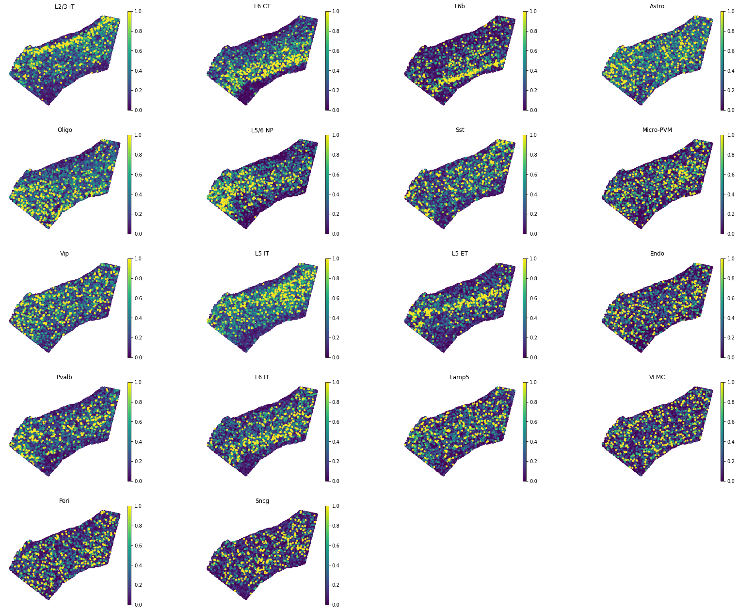
• The most common application for mapping single cell data onto space is to transfer the cell type annotations onto space.

• This is dona via plot_cell_annotation, which visualizes spatial probability maps of the annotation in the obs dataframe (here, the subclass_label field). You can set robust argument to True and at the same time set the perc argument to set the range to the colormap, which would help remove outliers.

• The following plots recover cortical layers of excitatory neurons and sparse patterns of glia cells. The boundaries of the cortex are defined by layer 6b (cell type L6b) and oligodendrocytes are found concentrated into sub-cortical region, as expected.

• Yet, the VLMC cell type patterns does not seem correct: VLMC cells are clustered in the first cortical layer, whereas here are sparse in the ROI. This usually means that either (1) we have not used good marker genes for VLMC cells in our training genes (2) the present marker genes are very sparse in the spatial data, therefore they don’t contain good mapping signal.

tg.project_cell_annotations(ad_map, ad_sp, annotation='subclass_label')
annotation_list = list(pd.unique(ad_sc.obs['subclass_label']))
tg.plot_cell_annotation_sc(ad_sp, annotation_list,x='x', y='y',spot_size= 50, scale_factor=2,perc=0.02)

INFO:root:spatial prediction dataframe is saved in `obsm` `tangram_ct_pred` of the spatial AnnData.

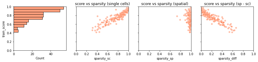
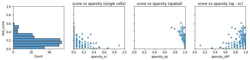
• Let’s try to get a deeper sense of how good this mapping is. A good helper is plot_training_scores which gives us four panels:

  • The first panels is a histogram of the simlarity score for each training gene. Most genes are mapped with very high similarity (> .9) although few of them have score ~.5. We would like to understand why for these genes the score is lower.

  • The second panel shows that there is a neat correlation between the training score of a gene (y-axis) and the sparsity of that gene in the snRNA-seq data (x-axis). Each dot is a training gene. The trend is that the sparser the gene the higher the score: this usually happens because very sparse gene are easier to map, as their pattern is matched by placing a few “jackpot cells” in the right spots.

  • The third panel is similar to the second one, but contains the gene sparsity of the spatial data. Spatial data are usually more sparse than single cell data, a discrepancy which is often responsible for low quality mapping.

  • In the last panel, we show the training scores as a function of the difference in sparsity between the dataset. For genes with comparable sparsity, the mapped gene expression is very similar to that in the spatial data. However, if a gene is quite sparse in one dataset (typically, the spatial data) but not in other, the mapping score is lower. This occurs as Tangram cannot properly matched the gene pattern because of inconsistent amount of dropouts between the datasets.

tg.plot_training_scores(ad_map, bins=10, alpha=.5)

• Although the above plots give us a summary of scores at single-gene level, we would need to know which are the genes are mapped with low scores.

• These information can be access from the dataframe .uns['train_genes_df'] from the mapping results; this is the dataframe used to build the four plots above.

• We want to inspect gene expression of training genes mapped with low scores, to understand the quality of mapping.

• First, we need to generate “new spatial data” using the mapped single cell: this is done via project_genes.

• The function accepts as input a mapping (adata_map) and corresponding single cell data (adata_sc).

• The result is a voxel-by-gene AnnData, formally similar to ad_sp, but containing gene expression from the mapped single cell data rather than Slide-seq.

ad_ge = tg.project_genes(adata_map=ad_map, adata_sc=ad_sc)
ad_ge

AnnData object with n_obs × n_vars = 9852 × 26496
    obs: 'orig.ident', 'nCount_RNA', 'nFeature_RNA', 'x', 'y', 'uniform_density', 'rna_count_based_density'
    var: 'n_cells', 'sparsity', 'is_training'
    uns: 'training_genes', 'overlap_genes'

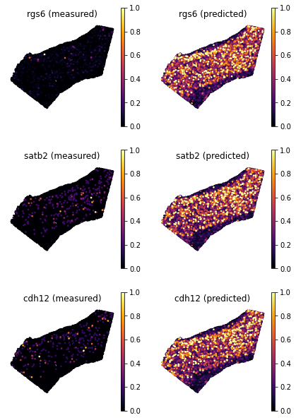
• We now choose a few training genes mapped with low score.

genes = ['rgs6', 'satb2',  'cdh12']
ad_map.uns['train_genes_df'].loc[genes]

	train_score	sparsity_sc	sparsity_sp	sparsity_diff
rgs6	0.462164	0.305172	0.941941	0.636769
satb2	0.501113	0.455904	0.969549	0.513645
cdh12	0.417188	0.384889	0.972594	0.587705

• To visualize gene patterns, we use the helper plot_genes. This function accepts two voxel-by-gene AnnData: the actual spatial data (adata_measured), and a Tangram spatial prediction (adata_predicted). The function returns gene expression maps from the two spatial AnnData on the genes genes.

• As expected, the predited gene expression is less sparse albeit the main patterns are captured. For these genes, we trust more the mapped gene patterns, as Tangram “corrects” gene expression by aligning in space less sparse data.

tg.plot_genes_sc(genes, adata_measured=ad_sp, adata_predicted=ad_ge, spot_size=50,scale_factor=0.1, perc=0.02, return_figure=False)

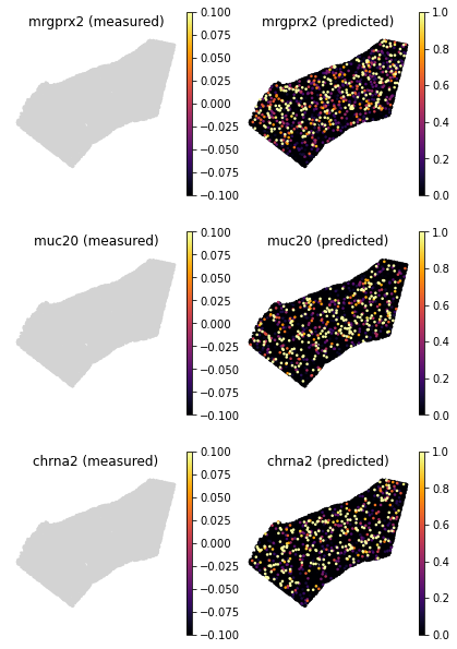
• An even stronger example is found in genes that are not detected in the spatial data, but are detected in the single cell data. They are removed before training with pp_adatas function. But tangram could still generate insight on how the spatial patterns look like.

genes=['mrgprx2', 'muc20', 'chrna2']
tg.plot_genes_sc(genes, adata_measured=ad_sp, adata_predicted=ad_ge, spot_size=50, scale_factor=0.1, perc=0.02, return_figure=False)

• So far, we only inspected genes used to align the data (training genes), but the mapped single cell data, ad_ge contains the whole transcriptome. That includes more than 26k test genes.

(ad_ge.var.is_training == False).sum()

26247

• We can use plot_genes to inspect gene expression of non training genes. This is an essential step as prediction of gene expression is the how we validate mapping.

• Before doing that, it is convenient to compute the similarity scores of all genes, which can be done by compare_spatial_geneexp. This function accepts two spatial AnnDatas (ie voxel-by-gene), and returns a dataframe with simlarity scores for all genes. Training genes are flagged by the Boolean field is_training.

• If we also pass single cell AnnData to compare_spatial_geneexp function like below, a dataframe with additional sparsity columns - sparsity_sc (single cell data sparsity) and sparsity_diff (spatial data sparsity - single cell data sparsity) will return. This is required if we want to call plot_test_scores function later with the returned datafrme from compare_spatial_geneexp function.

df_all_genes = tg.compare_spatial_geneexp(ad_ge, ad_sp, ad_sc)
df_all_genes

	score	is_training	sparsity_sp	sparsity_sc	sparsity_diff
igf2	9.996735e-01	True	0.994011	0.999924	-0.005913
chodl	9.967118e-01	True	0.999086	0.999016	0.000070
5031425f14rik	9.963596e-01	True	0.999594	0.998789	0.000805
car3	9.943125e-01	True	0.999695	0.999016	0.000679
scgn	9.935710e-01	True	0.999898	0.999205	0.000693
...	...	...	...	...	...
gm3376	1.477303e-08	False	0.999898	0.999962	-0.000064
gm21317	1.057379e-08	False	0.999898	0.999962	-0.000064
sprr2d	9.872679e-09	False	0.999898	0.999962	-0.000064
cd69	7.458404e-09	False	0.999898	0.999962	-0.000064
cyp1a2	7.139468e-09	False	0.999898	0.999962	-0.000064

18000 rows × 5 columns

• The plot below give us a summary of scores at single-gene level for test genes

tg.plot_auc(df_all_genes)

<Figure size 432x288 with 0 Axes>

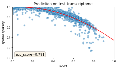
• Let’s plot the scores of the test genes and see how they compare to the training genes. Following the strategy in the previous plots, we visualize the scores as a function of the sparsity of the spatial data.

• (We have not wrapped this call into a function yet).

• Again, sparser genes in the spatial data are predicted with low scores, which is due to the presence of dropouts in the spatial data.

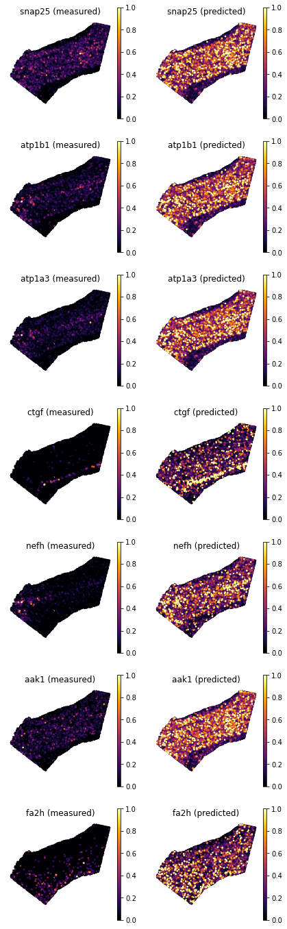
• Let’s choose a few test genes with varied scores and compared predictions vs measured gene expression.

genes = ['snap25', 'atp1b1', 'atp1a3', 'ctgf', 'nefh', 'aak1', 'fa2h', ]
df_all_genes.loc[genes]

	score	is_training	sparsity_sp	sparsity_sc	sparsity_diff
snap25	0.897492	False	0.402253	0.120048	0.282205
atp1b1	0.824424	False	0.579984	0.175778	0.404205
atp1a3	0.753856	False	0.658343	0.319587	0.338757
ctgf	0.585824	False	0.981628	0.948243	0.033386
nefh	0.536002	False	0.909156	0.916083	-0.006928
aak1	0.538055	False	0.868047	0.179713	0.688334
fa2h	0.363725	False	0.972493	0.860845	0.111648

• We can use again plot_genes to visualize gene patterns.

• Interestingly, the agreement for genes Atp1b1 or Apt1a3, seems less good than that for Ctgf and Nefh, despite the scores are higher for the former genes. This is because even though the latter gene patterns are localized correctly, their expression values are not so well correlated (for instance, in Ctgf the “bright yellow spot” is in different part of layer 6b). In contrast, for Atpb1 the gene expression pattern is largely recover, even though the overall gene expression in the spatial data is more dim.

tg.plot_genes_sc(genes, adata_measured=ad_sp, adata_predicted=ad_ge, spot_size=50,scale_factor=0.1, perc=0.02, return_figure=False)

---

Leave-One-Out Cross Validation (LOOCV)

• If number of genes is small, Leave-One-Out cross validation (LOOCV) is supported in Tangram to evaluate mapping performance.

• LOOCV supported by Tangram:

  • Assume the number of genes we have in the dataset is N.

  • LOOCV would iterate over and map on the genes dataset N times.

  • Each time it hold out one gene as test gene (1 test gene) and trains on the rest of all genes (N-1 training genes).

  • After all trainings are done, average test/train score will be computed to evaluate the mapping performance.

• Assume all genes we have is the training genes in the example above. Here we demo the LOOCV mapping at cluster level.

• Restart the kernel and load single cell, spatial and gene markers data

• Run pp_adatas to prepare data for mapping

import os, sys
import numpy as np
import pandas as pd
import matplotlib.pyplot as plt
import scanpy as sc
import torch
import tangram as tg

path = os.path.join('data', 'slideseq_MOp_1217.h5ad')
ad_sp = sc.read_h5ad(path)

path = os.path.join('data','mop_sn_tutorial.h5ad')
ad_sc = sc.read_h5ad(path)
sc.pp.normalize_total(ad_sc)

df_genes = pd.read_csv('data/MOp_markers.csv', index_col=0)
markers = np.reshape(df_genes.values, (-1, ))
markers = list(markers)

tg.pp_adatas(ad_sc, ad_sp, genes=markers)

INFO:root:249 training genes are saved in `uns``training_genes` of both single cell and spatial Anndatas.
INFO:root:18000 overlapped genes are saved in `uns``overlap_genes` of both single cell and spatial Anndatas.
INFO:root:uniform based density prior is calculated and saved in `obs``uniform_density` of the spatial Anndata.
INFO:root:rna count based density prior is calculated and saved in `obs``rna_count_based_density` of the spatial Anndata.

cv_dict, ad_ge_cv, df = tg.cross_val(ad_sc,
                                     ad_sp,
                                     device='cuda:0',
                                     mode='clusters',
                                     cv_mode='loo',
                                     num_epochs=1000,
                                     cluster_label='subclass_label',
                                     return_gene_pred=True,
                                     verbose=False,
                                     )

100%|█████████████████████████████████████████| 249/249 [22:51<00:00,  5.51s/it]

cv avg test score 0.185
cv avg train score 0.296

• cross_val function will return cv_dict and ad_ge_cv and df_test_genes in LOOCV mode. cv_dict contains the average score for cross validation, ad_ge_cv stores the predicted expression value for each gene, and df_test_genes contains scores and sparsity for each test genes.

cv_dict

{'avg_test_score': 0.1850259, 'avg_train_score': 0.29603068225355034}

• We can use plot_test_scores to display an overview of the cross validation test scores of each gene vs. sparsity.

tg.plot_test_scores(df, bins=10, alpha=.7)

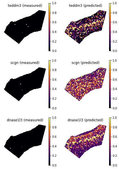
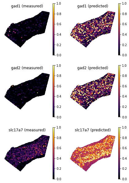
• Now, let’s compare a few genes between their ground truth and cross-validation predicted spatial pattern by calling the function plot_genes

ad_ge_cv.var.sort_values(by='test_score', ascending=False)

	test_score
gad1	0.612823
gad2	0.538168
slc17a7	0.507538
vtn	0.503739
pvalb	0.498329
...	...
5031425f14rik	0.015661
prok2	0.008919
teddm3	0.003758
scgn	0.002896
dnase1l3	0.000652

249 rows × 1 columns

ranked_genes = list(ad_ge_cv.var.sort_values(by='test_score', ascending=False).index.values)
top_genes = ranked_genes[:3]
bottom_genes = ranked_genes[-3:]

tg.plot_genes_sc(genes=top_genes, adata_measured=ad_sp, adata_predicted=ad_ge_cv, x = 'x', y='y',spot_size=50,scale_factor=0.1, perc=0.02, return_figure=False)

tg.plot_genes_sc(genes=bottom_genes, adata_measured=ad_sp, adata_predicted=ad_ge_cv,x='x', y='y', spot_size=50,scale_factor=0.1, perc=0.02, return_figure=False)