Tutorial for spatial mapping using Tangram

• by Ziqing Lu luz21@gene.com and Tommaso Biancalani biancalt@gene.com.

• Last update: August 16th 2021

What is Tangram?

Tangram is a method for mapping single-cell (or single-nucleus) gene expression data onto spatial gene expression data. Tangram takes as input a single-cell dataset and a spatial dataset, collected from the same anatomical region/tissue type. Via integration, Tangram creates new spatial data by aligning the scRNAseq profiles in space. This allows to project every annotation in the scRNAseq (e.g. cell types, program usage) on space.

What do I use Tangram for?

The most common application of Tangram is to resolve cell types in space. Another usage is to correct gene expression from spatial data: as scRNA-seq data are less prone to dropout than (e.g.) Visium or Slide-seq, the “new” spatial data generated by Tangram resolve many more genes. As a result, we can visualize program usage in space, which can be used for ligand-receptor pair discovery or, more generally, cell-cell communication mechanisms. If cell segmentation is available, Tangram can be also used for deconvolution of spatial data. If your single cell are multimodal, Tangram can be used to spatially resolve other modalities, such as chromatin accessibility.

---

Frequently Asked Questions about Tangram

How is Tangram different, than all the other deconvolution/mapping method?

• Validation. Most methods “validate” mappings by looking at known patterns or proportion of cell types. These are good sanity checks, but are hardly useful when mapping is used for discovery. In Tangram, mappings are validated by inspective the predictions of holdout genes (test transcriptome).

My scRNAseq/spatial data come from different samples. Can I still use Tangram?

• Yes. There is a clever variation invented by Sten Linnarsson, which consists of mapping average cells of a certain cell type, rather than single cells. This method is much faster, and smooths out variation in biological signal from different samples via averaging. However, it requires annotated scRNA-seq, sacrifices resolving biological variability at single-cell level. To map this way, pass mode=cluster.

Does Tangram only work on mouse brain data?

• No. The original manuscript focused on mouse brain data b/c was funded by BICCN. We subsequently used Tangram for mapping lung, kidney and cancer tissue. If mapping doesn’t work for your case, that is hardly due to the complexity of the tissue.

Why doesn’t Tangram have hypotheses on the underlying model?

• Most models used in biology are probabilistic: they assume that data are generated according to a certain probability distribution, hence the hypothesis. But Tangram doesn’t work that way: the hypothesis is that scRNA-seq and spatial data are generated with the same process (i.e. same biology) regardless of the process.

Where do I learn more about Tangram?

• Check out our documentation for learning more about the method, or our GitHub repo for the latest version of the code. Tangram has been released in :cite:`tangram`.

---

Setting up

Tangram is based on pytorch, scanpy and (optionally but highly-recommended) squidpy - this tutorial is designed to work with squidy. You can also check this tutorial, prior to integration with squidpy.

• To run the notebook locally, create a conda environment as conda env create -f tangram_environment.yml using our YAML file.

• This notebook is based on squidpy v1.1.0.

import scanpy as sc
import squidpy as sq
import numpy as np
import pandas as pd
from anndata import AnnData
import pathlib
import matplotlib.pyplot as plt
import matplotlib as mpl
import skimage
import seaborn as sns
import tangram as tg

sc.logging.print_header()
print(f"squidpy=={sq.__version__}")

%load_ext autoreload
%autoreload 2
%matplotlib inline

scanpy==1.8.1 anndata==0.7.6 umap==0.5.1 numpy==1.19.1 scipy==1.5.2 pandas==1.3.4 scikit-learn==0.24.2 statsmodels==0.12.2 python-igraph==0.9.8 pynndescent==0.5.4
squidpy==1.1.2

Loading datasets

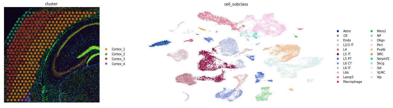
Load public data available in Squidpy, from mouse brain cortex. Single cell data are stored in adata_sc. Spatial data, in adata_st.

adata_st = sq.datasets.visium_fluo_adata_crop()
adata_st = adata_st[
    adata_st.obs.cluster.isin([f"Cortex_{i}" for i in np.arange(1, 5)])
].copy()
img = sq.datasets.visium_fluo_image_crop()

adata_sc = sq.datasets.sc_mouse_cortex()

We subset the crop of the mouse brain to only contain clusters of the brain cortex. The pre-processed single cell dataset was taken from :cite:`tasic2018shared` and pre-processed with standard scanpy functions.

Let’s visualize both spatial and single-cell datasets.

adata_st.obs

	in_tissue	array_row	array_col	n_genes_by_counts	log1p_n_genes_by_counts	total_counts	log1p_total_counts	pct_counts_in_top_50_genes	pct_counts_in_top_100_genes	pct_counts_in_top_200_genes	pct_counts_in_top_500_genes	total_counts_MT	log1p_total_counts_MT	pct_counts_MT	n_counts	leiden	cluster
AAATGGCATGTCTTGT-1	1	13	69	5191	8.554874	15977.0	9.678968	20.629655	26.757213	34.743694	48.889028	0.0	0.0	0.0	15977.0	0	Cortex_1
AACAACTGGTAGTTGC-1	1	28	42	5252	8.566555	16649.0	9.720165	20.481711	26.277855	34.092138	48.201093	0.0	0.0	0.0	16649.0	0	Cortex_1
AACAGGAAATCGAATA-1	1	15	67	6320	8.751633	23375.0	10.059465	17.929412	23.850267	32.077005	45.963636	0.0	0.0	0.0	23375.0	0	Cortex_1
AACCCAGAGACGGAGA-1	1	15	39	3659	8.205218	9229.0	9.130215	25.939972	31.964460	39.885145	53.212699	0.0	0.0	0.0	9229.0	1	Cortex_2
AACCGTTGTGTTTGCT-1	1	12	64	4512	8.414717	12679.0	9.447782	21.839262	28.038489	36.209480	50.540263	0.0	0.0	0.0	12679.0	0	Cortex_1
...	...	...	...	...	...	...	...	...	...	...	...	...	...	...	...	...	...
TTGGATTGGGTACCAC-1	1	17	55	4980	8.513386	15381.0	9.640953	21.038944	27.059359	35.114752	49.197061	0.0	0.0	0.0	15381.0	0	Cortex_1
TTGGCTCGCATGAGAC-1	1	23	37	4620	8.438366	13193.0	9.487517	20.609414	26.445842	34.063519	48.442356	0.0	0.0	0.0	13193.0	5	Cortex_3
TTGTATCACACAGAAT-1	1	12	74	6120	8.719481	21951.0	9.996614	18.199626	24.235798	32.440436	46.663022	0.0	0.0	0.0	21951.0	0	Cortex_1
TTGTGGCCCTGACAGT-1	1	18	60	4971	8.511577	14779.0	9.601030	21.381690	27.924758	36.213546	49.780093	0.0	0.0	0.0	14779.0	0	Cortex_1
TTGTTAGCAAATTCGA-1	1	22	42	4820	8.480737	14396.0	9.574775	20.595999	26.674076	34.655460	48.624618	0.0	0.0	0.0	14396.0	5	Cortex_3

324 rows × 17 columns

fig, axs = plt.subplots(1, 2, figsize=(20, 5))
sc.pl.spatial(
    adata_st, color="cluster", alpha=0.7, frameon=False, show=False, ax=axs[0]
)
sc.pl.umap(
    adata_sc, color="cell_subclass", size=10, frameon=False, show=False, ax=axs[1]
)
plt.tight_layout()

---

Tangram learns a spatial alignment of the single cell data by looking at a subset of genes, specified by the user, called the training genes. Training genes need to bear interesting signal and to be measured with high quality. Typically, we choose the training genes are 100-1000 differentially expressedx genes, stratified across cell types. Sometimes, we also use the entire transcriptome, or perform different mappings using different set of training genes to see how much the result change.

Tangram fits the scRNA-seq profiles on space using a custom loss function based on cosine similarity. The method is summarized in the sketch below:

Pre-processing

For this case, we use 1401 marker genes as training genes.

sc.tl.rank_genes_groups(adata_sc, groupby="cell_subclass", use_raw=False)
markers_df = pd.DataFrame(adata_sc.uns["rank_genes_groups"]["names"]).iloc[0:100, :]
markers = list(np.unique(markers_df.melt().value.values))
len(markers)

WARNING: Default of the method has been changed to 't-test' from 't-test_overestim_var'

1401

We prepares the data using pp_adatas, which does the following: - Takes a list of genes from user via the genes argument. These genes are used as training genes. - Annotates training genes under the training_genes field, in uns dictionary, of each AnnData. - Ensure consistent gene order in the datasets (Tangram requires that the the \(j\)-th column in each matrix correspond to the same gene). - If the counts for a gene are all zeros in one of the datasets, the gene is removed from the training genes. - If a gene is not present in both datasets, the gene is removed from the training genes.

tg.pp_adatas(adata_sc, adata_st, genes=markers)

INFO:root:1280 training genes are saved in `uns``training_genes` of both single cell and spatial Anndatas.
INFO:root:14785 overlapped genes are saved in `uns``overlap_genes` of both single cell and spatial Anndatas.
INFO:root:uniform based density prior is calculated and saved in `obs``uniform_density` of the spatial Anndata.
INFO:root:rna count based density prior is calculated and saved in `obs``rna_count_based_density` of the spatial Anndata.

Two datasets contain 1280 training genes of the 1401 originally provided, as some training genes have been removed.

Find alignment

To find the optimal spatial alignment for scRNA-seq profiles, we use the map_cells_to_space function: - The function maps iteratively as specified by num_epochs. We typically interrupt mapping after the score plateaus. - The score measures the similarity between the gene expression of the mapped cells vs spatial data on the training genes. - The default mapping mode is mode='cells', which is recommended to run on a GPU. - Alternatively, one can specify mode='clusters' which averages the single cells beloning to the same cluster (pass annotations via cluster_label). This is faster, and is our chioce when scRNAseq and spatial data come from different specimens. - If you wish to run Tangram with a GPU, set device=cuda:0 otherwise use the set device=cpu. - density_prior specifies the cell density within each spatial voxel. Use uniform if the spatial voxels are at single cell resolution (ie MERFISH). The default value, rna_count_based, assumes that cell density is proportional to the number of RNA molecules.

ad_map = tg.map_cells_to_space(adata_sc, adata_st,
    mode="cells",
#     mode="clusters",
#     cluster_label='cell_subclass',  # .obs field w cell types
    density_prior='rna_count_based',
    num_epochs=500,
    # device="cuda:0",
    device='cpu',
)

INFO:root:Allocate tensors for mapping.
INFO:root:Begin training with 1280 genes and rna_count_based density_prior in cells mode...
INFO:root:Printing scores every 100 epochs.

Score: 0.613, KL reg: 0.001
Score: 0.733, KL reg: 0.000
Score: 0.736, KL reg: 0.000
Score: 0.737, KL reg: 0.000
Score: 0.737, KL reg: 0.000

INFO:root:Saving results..

The mapping results are stored in the returned AnnData structure, saved as ad_map, structured as following: - The cell-by-spot matrix X contains the probability of cell i to be in spot j. - The obs dataframe contains the metadata of the single cells. - The var dataframe contains the metadata of the spatial data. - The uns dictionary contains a dataframe with various information about the training genes (saved as train_genes_df).

Cell type maps

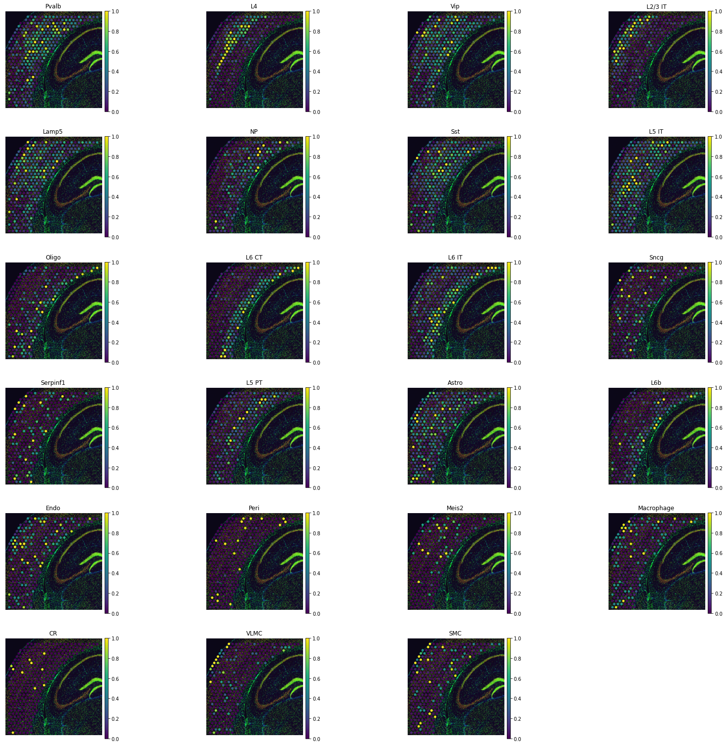
To visualize cell types in space, we invoke project_cell_annotation to transfer the annotation from the mapping to space. We can then call plot_cell_annotation to visualize it. You can set the perc argument to set the range to the colormap, which would help remove outliers.

ad_map

AnnData object with n_obs × n_vars = 21697 × 324
    obs: 'sample_name', 'organism', 'donor_sex', 'cell_class', 'cell_subclass', 'cell_cluster', 'n_genes_by_counts', 'log1p_n_genes_by_counts', 'total_counts', 'log1p_total_counts', 'pct_counts_in_top_50_genes', 'pct_counts_in_top_100_genes', 'pct_counts_in_top_200_genes', 'pct_counts_in_top_500_genes', 'total_counts_mt', 'log1p_total_counts_mt', 'pct_counts_mt', 'n_counts'
    var: 'in_tissue', 'array_row', 'array_col', 'n_genes_by_counts', 'log1p_n_genes_by_counts', 'total_counts', 'log1p_total_counts', 'pct_counts_in_top_50_genes', 'pct_counts_in_top_100_genes', 'pct_counts_in_top_200_genes', 'pct_counts_in_top_500_genes', 'total_counts_MT', 'log1p_total_counts_MT', 'pct_counts_MT', 'n_counts', 'leiden', 'cluster', 'uniform_density', 'rna_count_based_density'
    uns: 'train_genes_df', 'training_history'

tg.project_cell_annotations(ad_map, adata_st, annotation="cell_subclass")
annotation_list = list(pd.unique(adata_sc.obs['cell_subclass']))
tg.plot_cell_annotation_sc(adata_st, annotation_list,perc=0.02)

INFO:root:spatial prediction dataframe is saved in `obsm` `tangram_ct_pred` of the spatial AnnData.

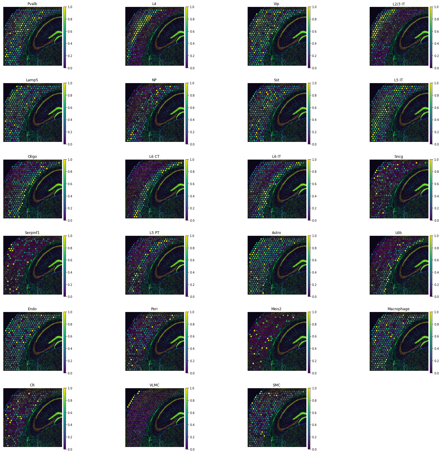
The first way to get a sense if mapping was successful is to look for known cell type patterns. To get a deeper sense, we can use the helper plot_training_scores which gives us four panels:

tg.plot_training_scores(ad_map, bins=20, alpha=.5)

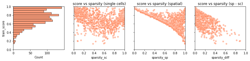
• The first panel is a histogram of the simlarity scores for each training gene.

• In the second panel, each dot is a training gene and we can observe the training score (y-axis) and the sparsity in the scRNA-seq data (x-axis) of each gene.

• The third panel is similar to the second one, but contains the gene sparsity of the spatial data. Spatial data are usually more sparse than single cell data, a discrepancy which is often responsible for low quality mapping.

• In the last panel, we show the training scores as a function of the difference in sparsity between the dataset. For genes with comparable sparsity, the mapped gene expression is very similar to that in the spatial data. However, if a gene is quite sparse in one dataset (typically, the spatial data) but not in other, the mapping score is lower. This occurs as Tangram cannot properly matched the gene pattern because of inconsistent amount of dropouts between the datasets.

Although the above plots give us a summary of scores at single-gene level, we would need to know which are the genes are mapped with low scores. These information are stored in the dataframe .uns['train_genes_df']; this is the dataframe used to build the four plots above.

ad_map.uns['train_genes_df']

	train_score	sparsity_sc	sparsity_sp	sparsity_diff
ppia	0.998200	0.000092	0.000000	-0.000092
ubb	0.997364	0.000092	0.000000	-0.000092
atp1b1	0.997066	0.014334	0.000000	-0.014334
tmsb4x	0.996971	0.002811	0.000000	-0.002811
ckb	0.996360	0.002765	0.000000	-0.002765
...	...	...	...	...
trpc5	0.194716	0.569203	0.981481	0.412278
cdyl2	0.189953	0.425911	0.981481	0.555570
cntnap5c	0.157349	0.608241	0.993827	0.385586
dlx1as	0.142076	0.587777	0.990741	0.402964
kcnh6	0.133051	0.379131	0.996914	0.617783

1280 rows × 4 columns

New spatial data via aligned single cells

If the mapping mode is 'cells', we can now generate the “new spatial data” using the mapped single cell: this is done via project_genes. The function accepts as input a mapping (adata_map) and corresponding single cell data (adata_sc). The result is a voxel-by-gene AnnData, formally similar to adata_st, but containing gene expression from the mapped single cell data rather than Visium. For downstream analysis, we always replace adata_st with the corresponding ad_ge.

ad_ge = tg.project_genes(adata_map=ad_map, adata_sc=adata_sc)
ad_ge

AnnData object with n_obs × n_vars = 324 × 36826
    obs: 'in_tissue', 'array_row', 'array_col', 'n_genes_by_counts', 'log1p_n_genes_by_counts', 'total_counts', 'log1p_total_counts', 'pct_counts_in_top_50_genes', 'pct_counts_in_top_100_genes', 'pct_counts_in_top_200_genes', 'pct_counts_in_top_500_genes', 'total_counts_MT', 'log1p_total_counts_MT', 'pct_counts_MT', 'n_counts', 'leiden', 'cluster', 'uniform_density', 'rna_count_based_density'
    var: 'mt', 'n_cells_by_counts', 'mean_counts', 'log1p_mean_counts', 'pct_dropout_by_counts', 'total_counts', 'log1p_total_counts', 'n_cells', 'highly_variable', 'highly_variable_rank', 'means', 'variances', 'variances_norm', 'sparsity', 'is_training'
    uns: 'cell_class_colors', 'cell_subclass_colors', 'hvg', 'neighbors', 'pca', 'umap', 'rank_genes_groups', 'training_genes', 'overlap_genes'

Let’s choose a few training genes mapped with low score, to try to understand why.

genes = ['rragb', 'trim17', 'eno1b']
ad_map.uns['train_genes_df'].loc[genes]

	train_score	sparsity_sc	sparsity_sp	sparsity_diff
rragb	0.358785	0.079919	0.867284	0.787365
trim17	0.201789	0.069641	0.959877	0.890236
eno1b	0.342446	0.022492	0.885802	0.863311

To visualize gene patterns, we use the helper plot_genes. This function accepts two voxel-by-gene AnnData: the actual spatial data (adata_measured), and a Tangram spatial prediction (adata_predicted). The function returns gene expression maps from the two spatial AnnData on the genes genes.

tg.plot_genes_sc(genes, adata_measured=adata_st, adata_predicted=ad_ge, perc=0.02)

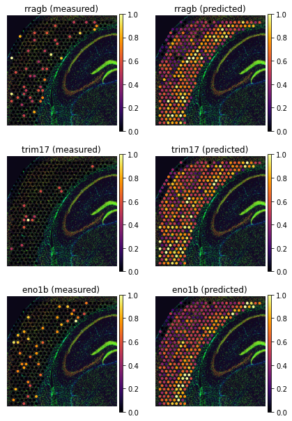
The above pictures explain the low training scores. Some genes are detected with very different levels of sparsity - typically they are much more sparse in the scRNAseq than in the spatial data. This is due to the fact that technologies like Visium are more prone to technical dropouts. Therefore, Tangram cannot find a good spatial alignment for these genes as the baseline signal is missing. However, so long as most training genes are measured with high quality, we can trust mapping and use Tangram prediction to correct gene expression. This is an imputation method which relies on entirely different premises than those in probabilistic models.

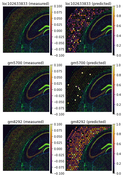
Another application is found by inspecting genes that are not detected in the spatial data, but are detected in the single cell data. They are removed before training with pp_adatas function, but Tangram can predict their expression.

genes=['loc102633833', 'gm5700', 'gm8292']
tg.plot_genes_sc(genes, adata_measured=adata_st, adata_predicted=ad_ge, perc=0.02)

• So far, we only inspected genes used to align the data (training genes), but the mapped single cell data, ad_ge contains the whole transcriptome. That includes more than 35k test genes.

(ad_ge.var.is_training == False).sum()

35546

We can use plot_genes to inspect gene expression of test genes as well. Inspecting the test transcriptome is an essential to validate mapping. At the same time, we need to be careful that some prediction might disagree with spatial data because of the technical droputs.

It is convenient to compute the similarity scores of all genes, which can be done by compare_spatial_geneexp. This function accepts two spatial AnnDatas (ie voxel-by-gene), and returns a dataframe with simlarity scores for all genes. Training genes are flagged by the boolean field is_training. If we also pass single cell AnnData to compare_spatial_geneexp function like below, a dataframe with additional sparsity columns - sparsity_sc (single cell data sparsity) and sparsity_diff (spatial data sparsity - single cell data sparsity) will return. This is required if we want to call plot_test_scores function later with the returned datafrme from compare_spatial_geneexp function.

df_all_genes = tg.compare_spatial_geneexp(ad_ge, adata_st, adata_sc)
df_all_genes

	score	is_training	sparsity_sp	sparsity_sc	sparsity_diff
snap25	0.998238	False	0.000000	0.014610	-0.014610
ppia	0.998200	True	0.000000	0.000092	-0.000092
gapdh	0.998200	False	0.000000	0.000968	-0.000968
calm1	0.997942	False	0.000000	0.000369	-0.000369
calm2	0.997779	False	0.000000	0.001751	-0.001751
...	...	...	...	...	...
6330420h09rik	0.000014	False	0.996914	0.998894	-0.001980
1810010k12rik	0.000014	False	0.996914	0.999585	-0.002672
cckar	0.000013	False	0.996914	0.999309	-0.002395
chil3	0.000013	False	0.996914	0.998894	-0.001980
cyp3a13	0.000013	False	0.996914	0.998479	-0.001565

14785 rows × 5 columns

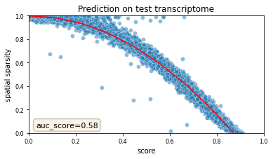
The prediction on test genes can be graphically visualized using plot_auc:

# sns.scatterplot(data=df_all_genes, x='score', y='sparsity_sp', hue='is_training', alpha=.5);  # for legacy
tg.plot_auc(df_all_genes);

<Figure size 432x288 with 0 Axes>

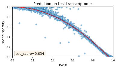
This above figure is the most important validation plot in *Tangram*. Each dot represents a gene; the x-axis indicates the score, and the y-axis the sparsity of that gene in the spatial data. Unsurprisingly, the genes predicted with low score represents very sparse genes in the spatial data, suggesting that the Tangram predictions correct expression in those genes. Note that curve observed above is typical of Tangram mappings: the area under that curve is the most reliable metric we use to evaluate mapping.

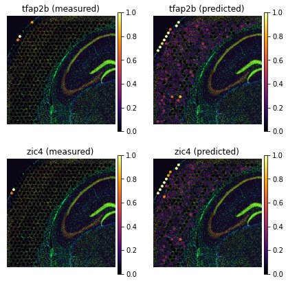
Let’s inspect a few predictions. Some of these genes are biologically sparse, but well predicted:

genes=['tfap2b', 'zic4']
tg.plot_genes_sc(genes, adata_measured=adata_st, adata_predicted=ad_ge, perc=0.02)

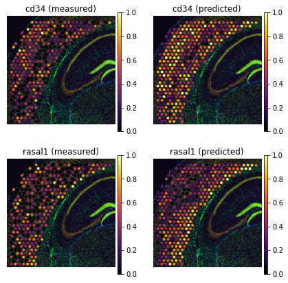
Some non-sparse genes present petterns, that Tangram accentuates:

genes = ['cd34', 'rasal1']
tg.plot_genes_sc(genes, adata_measured=adata_st, adata_predicted=ad_ge, perc=0.02)

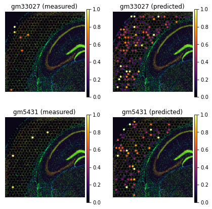
Finally, some unannotated genes have unknown function. These genes are often hardly detected in spatial data but Tangram provides prediction:

genes = ['gm33027', 'gm5431']
tg.plot_genes_sc(genes[:5], adata_measured=adata_st, adata_predicted=ad_ge, perc=0.02)

---

For untargeted spatial technologies, like Visium and Slide-seq, a spatial voxel may contain more than one cells. In these cases, it might be useful to disentangle gene expression into single cells - a process called deconvolution. Deconvolution is a requested feature, and also hard to obtain accurately with computational methods. If your goal is to study co-localization of cell types, we recommend you work with the spatial cell type maps instead. If your aim is discovery of cell-cell communication mechanisms, we suggest you compute gene programs, then use project_cell_annotations to spatially visualize program usage. To proceed with deconvolution anyways, see below.

In order to deconvolve cells, Tangram needs to know how many cells are present in each voxel. This is achieved by segmenting the cells on the corresponding histology, which squidpy makes possible with two lines of code: - squidpy.im.process applies smoothing as a pre-processing step. - squidpy.im.segment computes segmentation masks with watershed algorithm.

Note that some technologies, like Slide-seq, currently do not allow staining the same slide of tissue on which genes are profiled. For these data, you can still attempt a deconvolution by estimating cell density in a rough way - often we just pass a uniform prior. Finally, note that deconvolutions are hard to validate, as we do not have ground truth spatially-resolved single cells.

sq.im.process(img=img, layer="image", method="smooth")
sq.im.segment(
    img=img,
    layer="image_smooth",
    method="watershed",
    channel=0,
)

Let’s visualize the segmentation results for an inset

inset_y = 1500
inset_x = 1700
inset_sy = 400
inset_sx = 500

fig, axs = plt.subplots(1, 3, figsize=(30, 10))
sc.pl.spatial(
    adata_st, color="cluster", alpha=0.7, frameon=False, show=False, ax=axs[0], title=""
)
axs[0].set_title("Clusters", fontdict={"fontsize": 20})
sf = adata_st.uns["spatial"]["V1_Adult_Mouse_Brain_Coronal_Section_2"]["scalefactors"][
    "tissue_hires_scalef"
]
rect = mpl.patches.Rectangle(
    (inset_y * sf, inset_x * sf),
    width=inset_sx * sf,
    height=inset_sy * sf,
    ec="yellow",
    lw=4,
    fill=False,
)
axs[0].add_patch(rect)

axs[0].axes.xaxis.label.set_visible(False)
axs[0].axes.yaxis.label.set_visible(False)

axs[1].imshow(
    img["image"][inset_y : inset_y + inset_sy, inset_x : inset_x + inset_sx, 0, 0]
    / 65536,
    interpolation="none",
)
axs[1].grid(False)
axs[1].set_xticks([])
axs[1].set_yticks([])
axs[1].set_title("DAPI", fontdict={"fontsize": 20})

crop = img["segmented_watershed"][
    inset_y : inset_y + inset_sy, inset_x : inset_x + inset_sx
].values.squeeze(-1)
crop = skimage.segmentation.relabel_sequential(crop)[0]
cmap = plt.cm.plasma
cmap.set_under(color="black")
axs[2].imshow(crop, interpolation="none", cmap=cmap, vmin=0.001)
axs[2].grid(False)
axs[2].set_xticks([])
axs[2].set_yticks([])
axs[2].set_title("Nucleous segmentation", fontdict={"fontsize": 20});

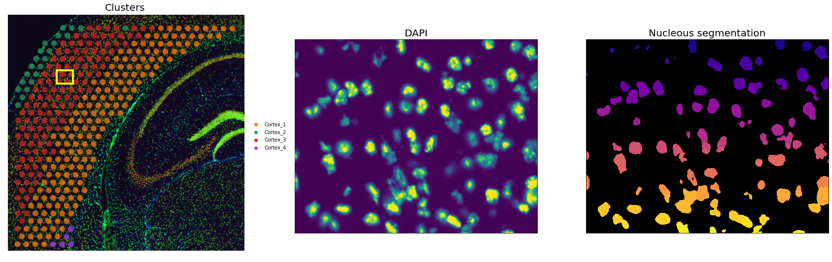
Comparison between DAPI and mask confirms the quality of the segmentation. We then need to extract some image features useful for the deconvolution task downstream. Specifically: - the number of unique segmentation objects (i.e. nuclei) under each spot. - the coordinates of the centroids of the segmentation object.

# define image layer to use for segmentation
features_kwargs = {
    "segmentation": {
        "label_layer": "segmented_watershed",
        "props": ["label", "centroid"],
        "channels": [1, 2],
    }
}
# calculate segmentation features
sq.im.calculate_image_features(
    adata_st,
    img,
    layer="image",
    key_added="image_features",
    features_kwargs=features_kwargs,
    features="segmentation",
    mask_circle=True,
)

100%|██████████| 324/324 [01:19<00:00,  4.09/s]

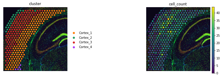
We can visualize the total number of objects under each spot with scanpy.

adata_st.obs["cell_count"] = adata_st.obsm["image_features"]["segmentation_label"]
sc.pl.spatial(adata_st, color=["cluster", "cell_count"], frameon=False)

Deconvolution via alignment

The rationale for deconvolving with Tangram, is to constrain the number of mapped single cell profiles. This is different that most deconvolution method. Specifically, we set them equal to the number of segmented cells in the histology, in the following way: - We pass mode='constrained'. This adds a filter term to the loss function, and a boolean regularizer. - We set target_count equal to the total number of segmented cells. Tangram will look for the best target_count cells to align in space. - We pass a density_prior, containing the fraction of cells per voxel.

ad_map = tg.map_cells_to_space(
    adata_sc,
    adata_st,
    mode="constrained",
    target_count=adata_st.obs.cell_count.sum(),
    density_prior=np.array(adata_st.obs.cell_count) / adata_st.obs.cell_count.sum(),
    num_epochs=1000,
#     device="cuda:0",
    device='cpu',
)

Score: 0.613, KL reg: 0.125, Count reg: 5724.304, Lambda f reg: 4490.422
Score: 0.698, KL reg: 0.012, Count reg: 1.051, Lambda f reg: 734.217
Score: 0.700, KL reg: 0.012, Count reg: 1.661, Lambda f reg: 243.458
Score: 0.701, KL reg: 0.012, Count reg: 0.286, Lambda f reg: 172.023
Score: 0.701, KL reg: 0.012, Count reg: 0.325, Lambda f reg: 143.205
Score: 0.701, KL reg: 0.012, Count reg: 0.129, Lambda f reg: 123.143
Score: 0.701, KL reg: 0.012, Count reg: 0.029, Lambda f reg: 107.319
Score: 0.701, KL reg: 0.012, Count reg: 0.530, Lambda f reg: 96.239
Score: 0.701, KL reg: 0.012, Count reg: 0.375, Lambda f reg: 90.205
Score: 0.701, KL reg: 0.012, Count reg: 0.081, Lambda f reg: 83.204

In the same way as before, we can plot cell type maps:

tg.project_cell_annotations(ad_map, adata_st, annotation="cell_subclass")
annotation_list = list(pd.unique(adata_sc.obs['cell_subclass']))
tg.plot_cell_annotation_sc(adata_st, annotation_list, perc=0.02)

We validate mapping by inspecting the test transcriptome:

ad_ge = tg.project_genes(adata_map=ad_map, adata_sc=adata_sc)
df_all_genes = tg.compare_spatial_geneexp(ad_ge, adata_st, adata_sc)
tg.plot_auc(df_all_genes);

<Figure size 432x288 with 0 Axes>

And here comes the key part, where we will use the results of the previous deconvolution steps. Previously, we computed the absolute numbers of unique segmentation objects under each spot, together with their centroids. Let’s extract them in the right format useful for Tangram. In the resulting dataframe, each row represents a single segmentation object (a cell). We also have the image coordinates as well as the unique centroid ID, which is a string that contains both the spot ID and a numerical index. Tangram provides a convenient function to export the mapping between spot ID and segmentation ID to adata.uns.

tg.create_segment_cell_df(adata_st)
adata_st.uns["tangram_cell_segmentation"].head()

	spot_idx	y	x	centroids
0	AAATGGCATGTCTTGT-1	5304.000000	731.000000	AAATGGCATGTCTTGT-1_0
1	AAATGGCATGTCTTGT-1	5320.947519	721.331554	AAATGGCATGTCTTGT-1_1
2	AAATGGCATGTCTTGT-1	5332.942342	717.447904	AAATGGCATGTCTTGT-1_2
3	AAATGGCATGTCTTGT-1	5348.865384	558.924248	AAATGGCATGTCTTGT-1_3
4	AAATGGCATGTCTTGT-1	5342.124989	567.208502	AAATGGCATGTCTTGT-1_4

We can use tangram.count_cell_annotation() to map cell types as result of the deconvolution step to putative segmentation ID.

tg.count_cell_annotations(
    ad_map,
    adata_sc,
    adata_st,
    annotation="cell_subclass",
)
adata_st.obsm["tangram_ct_count"].head()

	x	y	cell_n	centroids	Pvalb	L4	Vip	L2/3 IT	Lamp5	NP	...	L5 PT	Astro	L6b	Endo	Peri	Meis2	Macrophage	CR	VLMC	SMC
AAATGGCATGTCTTGT-1	641	5393	13	[AAATGGCATGTCTTGT-1_0, AAATGGCATGTCTTGT-1_1, A...	1	0	1	0	0	0	...	2	0	0	0	0	0	0	0	0	0
AACAACTGGTAGTTGC-1	4208	1672	16	[AACAACTGGTAGTTGC-1_0, AACAACTGGTAGTTGC-1_1, A...	1	0	4	0	2	1	...	1	0	0	0	0	0	0	0	0	0
AACAGGAAATCGAATA-1	1117	5117	28	[AACAGGAAATCGAATA-1_0, AACAGGAAATCGAATA-1_1, A...	1	1	3	0	2	0	...	0	0	1	0	1	1	0	0	0	0
AACCCAGAGACGGAGA-1	1101	1274	5	[AACCCAGAGACGGAGA-1_0, AACCCAGAGACGGAGA-1_1, A...	2	0	0	0	0	0	...	0	1	0	0	0	0	1	0	0	0
AACCGTTGTGTTTGCT-1	399	4708	7	[AACCGTTGTGTTTGCT-1_0, AACCGTTGTGTTTGCT-1_1, A...	2	1	0	0	0	0	...	1	0	0	2	0	0	0	0	0	1

5 rows × 27 columns

And finally export the results in a new AnnData object.

adata_segment = tg.deconvolve_cell_annotations(adata_st)
adata_segment.obs.head()

	y	x	centroids	cluster
0	5304.000000	731.000000	AAATGGCATGTCTTGT-1_0	Pvalb
1	5320.947519	721.331554	AAATGGCATGTCTTGT-1_1	Vip
2	5332.942342	717.447904	AAATGGCATGTCTTGT-1_2	Sst
3	5348.865384	558.924248	AAATGGCATGTCTTGT-1_3	L5 IT
4	5342.124989	567.208502	AAATGGCATGTCTTGT-1_4	L6 CT

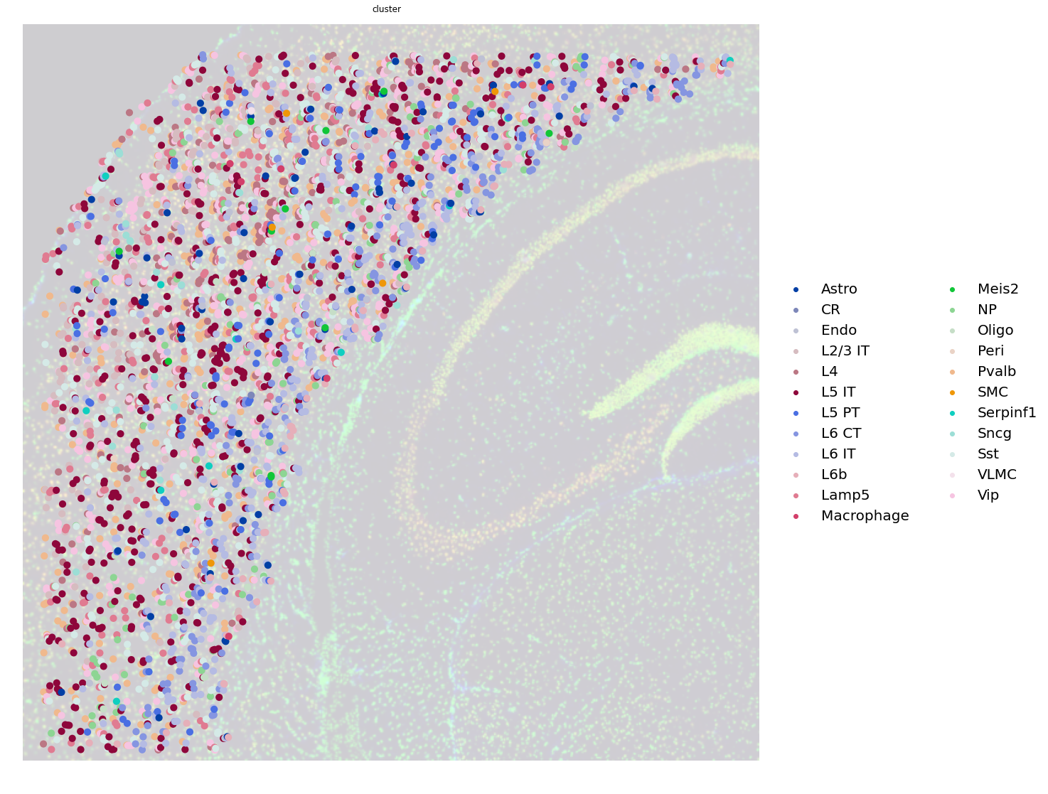
Note that the AnnData object does not contain counts, but only cell type annotations, as results of the Tangram mapping. Nevertheless, it’s convenient to create such AnnData object for visualization purposes. Below you can appreciate how each dot is now not a Visium spot anymore, but a single unique segmentation object, with the mapped cell type.

fig, ax = plt.subplots(1, 1, figsize=(20, 20))
sc.pl.spatial(
    adata_segment,
    color="cluster",
    size=0.4,
    show=False,
    frameon=False,
    alpha_img=0.2,
    legend_fontsize=20,
    ax=ax,
)

[<AxesSubplot:title={'center':'cluster'}, xlabel='spatial1', ylabel='spatial2'>]